Projects
Classifying Online Shopper’s Intention
Completed as Capstone Project at Springboard
If you would like to read this in one document, click on this link: Google Doc
Introduction
Online shopping is a huge and growing form of purchasing and represents a huge portion of B2C (Business to Customer) revenue. 69% of Americans have shopped online at some point (1), with an average revenue of $1804 per online shopper(2). 36% of Americans shop online at least once per month! Learning how and when shoppers will research and purchase goods online is important to businesses as they can use customer behavior insights to target advertising, marketing, and deals to potential customers to further increase their sales and revenue.
The Data
The dataset is taken from the UCI Machine Learning repository and features precleaned data for online websites. The data set is a set of 18 features: 10 numerical and 8 categorical. This dataset has 12,330 entries, split into 10,422 entries where the shoppers did not purchase and 1908 entries where the shoppers did purchase. Each entry is based on unique users in a 1-year period to avoid any trends specific to a specific campaign.
| Feature | Description |
|---|---|
| Administrative | This is the number of pages of this type (administrative) that the user visited. |
| Administrative_Duration | This is the amount of time spent in this category of pages. |
| Informational | This is the number of pages of this type (informational) that the user visited. |
| Informational_Duration | This is the amount of time spent in this category of pages. |
| ProductRelated | This is the number of pages of this type (product related) that the user visited. |
| ProductRelated_Duration | This is the variable measured. The Tenure is categorized into two subsets, 1: Households that own their house with a mortgage or loan. 2: Households that own their homes free and clear. |
| BounceRates | The percentage of visitors who enter the website through that page and exit without triggering any additional tasks. |
| ExitRates | The percentage of pageviews on the website that end at that specific page. |
| PageValues | The average value of the page averaged over the value of the target page and/or the completion of an eCommerce transaction. |
| SpecialDay | This value represents the closeness of the browsing date to special days or holidays (eg Mother's Day or Valentine's day) in which the transaction is more likely to be finalized. More information about how this value is calculated below. |
| Month | Contains the month the pageview occurred, in string form. |
| OperatingSystems | An integer value representing the operating system that the user was on when viewing the page. |
| Browser | An integer value representing the browser that the user was using to view the page. |
| Region | An integer value representing the browser that the user was using to view the page. |
| TrafficType | An integer value representing what type of traffic the user is categorized into. |
| VisitorType | A string representing whether a visitor is New Visitor, Returning Visitor, or Other. |
| Weekend | A boolean representing whether the session is on a weekend. |
| Revenue | A boolean representing whether or not the user completed the purchase. |
Exploratory Data Analysis
From exploratory data analysis we look for any issues with the data first. This datatset has been pruned by the UCI Machine Learning repository, so therefore has no null values. We confirm this by checking for nulls in our notebook.

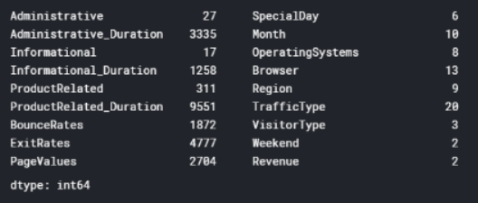
Then, we check to see the number of unique values for each feature.
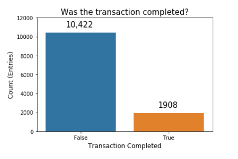
Our next step is to investigate our label feature. In this case it is “Revenue”, which is a boolean value representing whether or not the shopper made a purchase.We can see that the number of entries where the customer ended up not purchasing is much higher that the number of entries where the customer ended up completing a transaction. This makes sense, as a majority of normal online shopping ends without a purchase.
Feature Cleaning
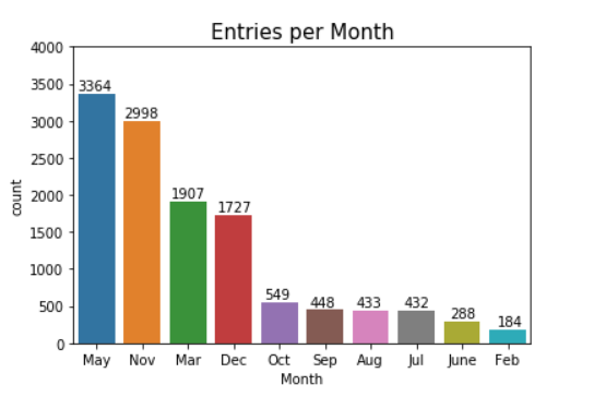
In order to prepare our data, we need to switch our labels to the correct format. We have a few features that need to be adjusted. First, we drop the month column. The 'Month' column only has 10 unique types, which indicates that it is missing two months of data. Each month has varying numbers of entries, which could unfairly bias our data to prefer classification by month. We can see below the distribution of each month in the 'Month' column. Additionally, time-sensitivity is already contained in the 'SpecialDay' column, which influences buying decisions, so the month column is slightly redundant.
We can see here that the 'Month' column is missing January and April. We can also see visually that several months have many samples (May, Nov) and a couple have very few samples (Feb, June). We will remove this column.
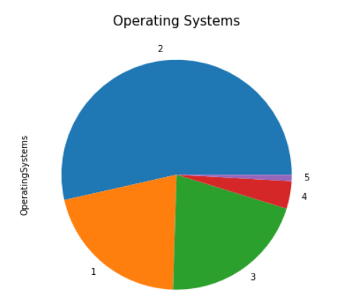
 Here we have the Operating Systems, labeled by number. Low-usage browsers have been consolidated into label '5'. We can see that a majority of users use operating system #2. Operating systems can indicate users of a sepcifc type of computer and may portray certain user archetypes (Windows users, Mac users, Linux users). For now, we will forgo usage of this column for our classifier.
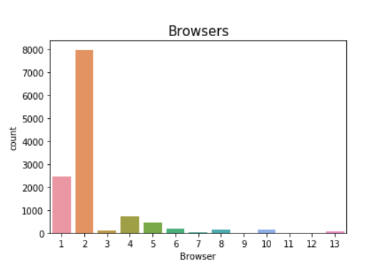
 Browser choice is even more polarizing than the Operating System. Here we see that a large majority of users use browser 2, with a smaller number of users using browser 1. All other browsers represent a small subsection of online users. We will not use this as it does not contribute much to our model.
There are several other columns that we leave out:
'Region': We leave regionality out because the regionality may be slightly tied to purchase likelihood, but we want to train our model on a smaller set of features if possible.
'TrafficType': We leave this column out because Traffic sources are not quite useful for classifying if a user will make a purchase. It usually aids website owners in gauging traffic sources and can assist with determining where they should invest in advertisement.
'Weekend':There is weak correlation between days of the week and online shopping.
This blog post asserts that Sundays and Mondays have the highest traffic for eCommerce, but only by 16% of weekly revenue, and mostly on Monday, which is not classified as a weekend.
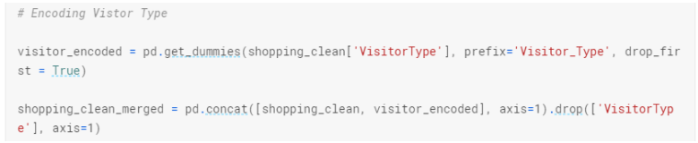
Our last step prior to creating a model is to encode our features that have more than two unique features into distinct columns that represent all choices in order to remove any ordinal information.
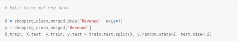
Finally, we split our training and test data.
Creating a Model
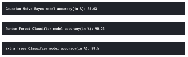
We first train three types of models using our training / testing data:
Naive Bayes, Random Forest and Extra Trees.
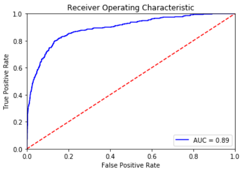
 In order to evaluate the performance of our model, we plot the ROC curve for our best model, which is the Random Forest Classifier.

Creating a Model
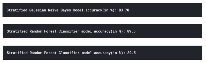
Because the training data is so heavily skewed in the direction of the 'No purchase made' category, we must stratify our training data so that the ratio of training labels is equal. We use the stratified shuffle split package included in the Sci-kit learn library to achieve this. We then reevaluate our three models:
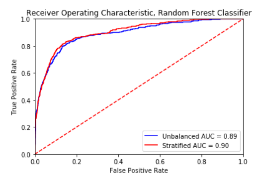
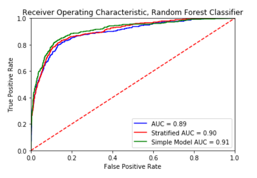
Once again, we plot the ROC curve. We can see that the performance is functionally identical, which means that our model is robust, and does not abuse the skewness of our Revenue label.
To best understand our model, we check feature importances for each feature in our model.
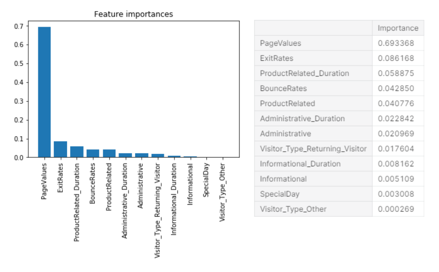 Taking a look at our feature importances, it is clear that the largest contributor to the model accuracy is Google’s PageValues. Seeing these feature importances, we want to simplify our model to only use features that may heavily contribute to our classification. Using our feature importance chart, we will take the top 5 most impactful features: PageValues, ExitRates, ProductRelated_Duration, BounceRates, ProductRelated. In addition, after creating the simplififed model, we want to measure the effectiveness of our model by using cross validation.
Creating a Simple Model
In order for us to create a simplified model, we canuse our feature importances, and only choose the top 5 most impactful features. These features are PageValues, ExitRates, ProductRelated_Duration, BounceRates, ProductRelated. In addition, in order to make sure that our model is robust, we will use k-fold cross validation over ten folds in order to evaluate whether our model is consistent.

We can see that throughout ten splits of the data, our model accuracy stays at around 90%, with a standard deviation of 0.01.
Now, we plot the ROC curve of our simplified model versus the other two preiterations.
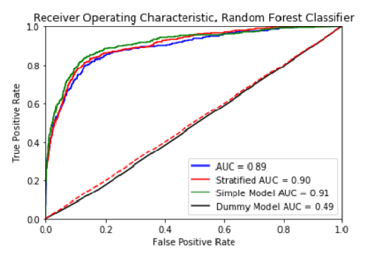
All three models seem to have similar performance. Now, we try a dummy classifier to compare results to see if the classifiers are producing better results than guessing. We can see here that a dummy classifier is only around 50% accurate, as expected.
Conclusion
Our model seems to be much more accurate than guessing. By using a random forest classifier, we are able to achieve approximately 90% accuracy. The dummy classifier seems to be right about 50% of the time, which we should expect to see, as it is making guesses based on the distribution of a stratified dataset. If we were to deploy this model, the most efficient model to select would be our simple model. The simple model performs similarly to our other models, and only bases its classification by five features.
The model we have created is a robust model, being able to make accurate predictions 90% of the time. We determined through 10-fold cross validation that our model is consistent.
Future Works
To further improve the model, we would need to diverge from the reliance on the Google analytics page score. At this point a majority of our model accuracy comes from this number. In addition, our dataset is very imbalanced, and despite stratifying our data and training it on stratified data, it would be in our best interest to bolster our dataset with examples where customers ended up purchasing.
This model is a minimum viable product. In order to use the model, we have to specify a data file to read and make predictions. In most online shopping situations, you would use this model to target advertisements or special campaigns to people who may not want to purchase a product in order to lift the conversion rate. Another way that you could use this model is to manage supply and demand by monitoring the conversion and success rate for their shoppers. By quantifying the likelihood of conversion, an online e-commerce store may be able to fine tune their price and products, as well as their user interface to optimize the success of their online store.