Projects
Senior Thesis
Completed May 2018, University of California, Irvine Department of Earth System Science, Primeau Lab
Predicting Carbon Export Using Satellite Data to Estimate Mean Planktonic Size and Sinking Speed
Abstract
The ocean sequesters carbon in the deep ocean via the production and sinking of particulate organic carbon from the surface. Understanding the sequestration of carbon by organic matter flux requires accurate prediction of the size-dependent sinking speeds of organic particles. Particle sinking speeds can be calculated using Stokes’ Law, which predicts sinking speed based on particle radius and density. Additionally, an extended model is used here to predict the sinking speeds of diatoms by accounting for the additional frustle of the diatom. We estimate global export of particulate organic carbon from the euphotic zone by combining estimated particle sinking speed and a satellite product of marine particle abundance. Seawater viscosity is computed from satellite derived sea surface temperature and sea surface salinity. Validation against in-situ particle flux data is relatively weak, pointing to directions for possible improvement of the model.
Introduction
The ocean is important to study because it is a crucial part of the world’s CO2 cycle. The biological pump is a process where phytoplankton particles sink and remineralize out of the well-lit mixed layer to the deep ocean and serves as a key method for the sequestration of atmospheric carbon. Estimating carbon export within the ocean is difficult, with studies predicting a large range of 5 to 12 Petagrams of carbon yearly exported from the euphotic zone (Siegel et al 2014). Creating new methods to measure and estimate the export of carbon is an important way to decrease the uncertainty in the carbon export estimate. Furthermore, sediment trap data of phytoplankton sinking speeds is sparse in space and time. Satellite data offers superior spatial and repetitive coverage, which motivates the creation of models that can estimate carbon export from satellite data. Satellite data has also recently been used to estimate the distribution of different particle size classes of phytoplankton in the ocean from backscattering, which is used to create an estimate of global carbon export.
Stokes Law and Predicting Sinking Speeds
A. Particle Size and Sinking Speed
i. Basic Stokes Law
Sinking speeds of phytoplankton are often estimated by Stokes’ law, which predicts sinking velocities that scale by an exponent of 2 in relation to its radius. Sinking plankton particles satisfy the prerequisites of Stokes’ Law, as they are small, slow moving spherical objects that move slowly in relation to its outside medium. Using a newer model predicts that diatoms, which synthesize approximately half of the ocean’s fixed carbon (Nelson et al 1995; Field et al 1998, cited within Miklasz et al 2010), may follow a more complex extended Stokes Law that accounts for the differing densities of diatomic components (Miklasz and Denny 2010).
The classic stokes model predicts that a sinking particle’s speed (U) is:
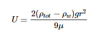
Where ρtot is the density of the particle, ρw is the density of the surrounding liquid (in this case water), r is the radius of the particle, g is the constant of gravitational acceleration (9.8 m s-2), and μ is the dynamic viscosity of surrounding liquid (water).The extended model presented by Miklasz and Denny (2010) assumes constants of ρw = 1023 kg m-3 and μ = 1.07 x 10⁻³ Pa s, which represents the density and dynamic viscosity of water at 20°C and 33 g L-1 salinity, respectively. Stokes’ law holds up for particles with small Reynolds numbers (Re < 1), which describes all particles mentioned in this paper. Since both dynamic viscosity and water’s density varies with temperature and salinity, it is important to consider both variables within our calculation. However, because the range at which water’s density varies with respect to temperature and salinity differences is so small, we can safely assume water to have a constant density of ρw ≈ 1023 kg m-3.
Since dynamic viscosity is a large factor in this equation (Fig. 1), we include the variation of dynamic viscosity within our calculation. Dynamic viscosity (μ) is a key variable in Stokes Law that is overlooked. Miklasz and Denny (2010) assume that dynamic viscosity remains constant. Dynamic viscosity depends on temperature and salinity, and is dominated by the effects of the former (Fig. 1). The effect of dynamic viscosity is very apparent over the relevant temperature range, with a 63% decrease in predicted sinking speed between temperatures T = 0 and T = 40. (Fig 2). In order to calculate the change in dynamic viscosity, we use a seawater toolbox that estimates dynamic viscosity of seawater given temperature and salinity (Sharqawy et al 2010). Using this basic Stokes’ law model, sinking speed ( “U” ) is estimated for diatoms with small, medium, and large radii, with values of 5 μm, 10 μm, and 20 μm, respectively (Fig. 3). The sinking velocity of each particle increases by an exponent of 2, which greatly overestimates the sinking speed of larger particles.
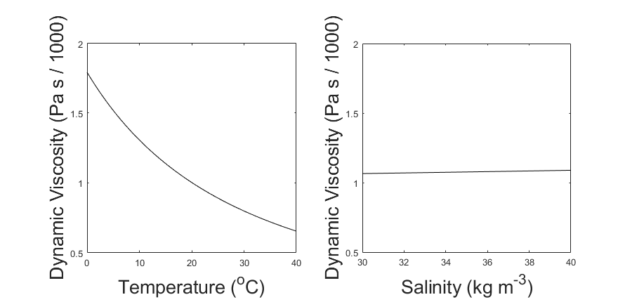 Figure 1: Variation in Dynamic Viscosity of Seawater (μ). Viscosity is plotted against temperature, while holding salinity constant at 35 kg m-3 (left). Viscosity is also plotted against salinity, while holding temperature constant at 20oC (right). Over the normal range of each variable, the change in viscosity is dominated by the effect of Temperature.
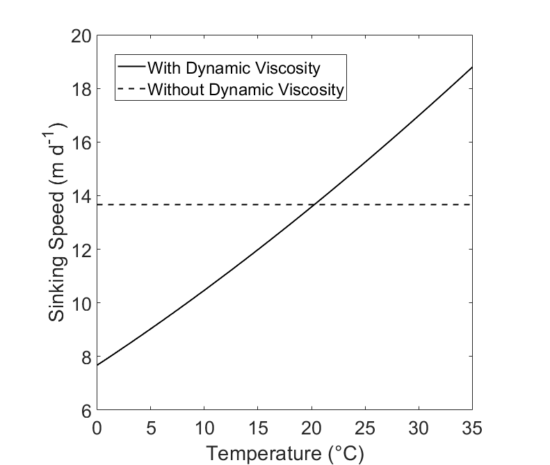 Figure 2: The hypothetical sinking speed (“U”) of two cells with identical structure, calculated with and without dynamic viscosity. The solid line (“With Dynamic Viscosity) represents a model that uses the effect of temperature as it increases from 0°C to 35°C. The dashed line (“Without Dynamic Viscosity”) represents a sinking The cell is plotted where r = 10 μm and has a uniform cell density of ρtot = 1800 kg m-3.
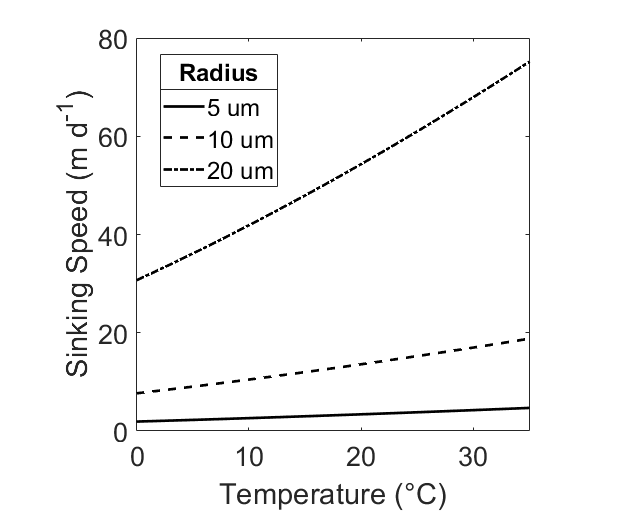
Figure 3: Sinking speed (U) in meters per day, calculated by Stokes’ Law. Hypothetical radius values of r = 5 μm (dashed), r = 10 μm (solid), and r = 20 μm (dot / dash) are displayed. Temperature range is 0oC ≤ T ≤35oC, Salinity S = 35 ppt, total cell density ρtot = 1800 kg m-3.
ii. Extended Stokes Model
Stokes Law is defined for a spherical particle with uniform density, which does not perfectly describe a diatom’s structure. A diatom may have a hard, dense silicate frustle as well as a less dense cytoplasmic core. Diatomic frustles may constitute up to 70% silica, which is much denser than water (2500 kg m-3). The cytoplasm is less directly studied, with no direct measurement. The density of cytoplasm is said to be in the range of 1030 to 1100 kg m-3 (Smayda 1970). Diatoms constitute mostly cytoplasm, with the frustle thickness usually contributing less than half of the diatom’s radius. Because of this, the diatom’s sinking speed is usually overestimated by the normal Stokes’ equation. The proposed extended Stokes’ theorem (Miklasz and Denny, 2010) assumes a spherical shape and accounts for diatom radius and frustle thickness to produce an estimate of sinking speed that more accurately reflects the density of the entire cell. For a diatom with a cell radius r = 10 μm, the basic model predicts a sinking speed of , while the extended model predicts a sinking speed of , using a frustle thickness of 1 μm; neither of the estimates account for dynamic viscosity (Fig. 4). Additionally, Figure 4 displays the difference in both models when dynamic viscosity changes between temperatures of 0ᵒC and 35ᵒC. The lower density of the cytoplasm causes the estimated sinking speed for the extended model to be approximately 60% lower when dynamic viscosity is held constant. Figure 5 displays sinking speed estimates of diatoms with different cytoplasmic and frustle densities, with radii r = 10 μm and frustle thickness 1 μm.
 Equation 2: The Extended Stokes’ Model. ρcyt represents the density of the cytoplasm, ρfr represents the density of the frustle, ρw represents the density of water, r is the radius of the diatom, t is the thickness of the diatom’s frustle, g = 9.8 m s-2, the gravitational constant, and μ is the dynamic viscosity of seawater.
Table 1 represents typical ranges of values for diatoms (Kostadinov et al 2009).

 Figure 4: Comparisons between Stokes Model and Extended Model. Temperature range is 0oC ≤ T ≤ 35oC, Salinity S = 35 ppt. The basic Stokes Model assumes a cell radius of r = 10 μm and a uniform cell density of ρtot = 1800 kg m-3 (“Stokes’ Model”). The Extended Model assumes a cell radius of r = 10 μm, a frustle thickness of t = 1 μm, a cytoplasm density of ρcyt =1065 kg m-3, and a frustle density of ρfr = 1800 kg m-3 (“Extended Model”). Each model is presented with and without the influence of dynamic viscosity.
 Figure 5: Comparison of Sinking Speed (U) of diatoms at different densities. Sinking Speeds are calculated using the Extended Model. The hypothetical diatoms have radius r = 10 and frustle thickness t = 1 μm
B. Global Maps of Important Environmental Variables that are measured by satellite (T, S, μ)
Dynamic viscosity is dependent on salinity and temperature. Using data gathered by satellites, we generate a yearly average sea surface salinity and sea surface temperature model. Sea surface salinity data is taken from the Aquarius satellite during the year 2012, using monthly averages at 1 degree resolution. Sea surface temperature data is taken from MODIS during the year 2012, using monthly averages at 1 degree resolution. Both sets of data are downloaded from the NASA OceanColor Website. A yearly average of both sea surface temperature and sea surface salinity is created using the data (Fig.6). Dynamic viscosity depends on the temperature and the salinity of seawater. Using both the sea surface salinity and the sea surface temperature data, a global map of the yearly average dynamic viscosity of the ocean is created (Fig. 7).

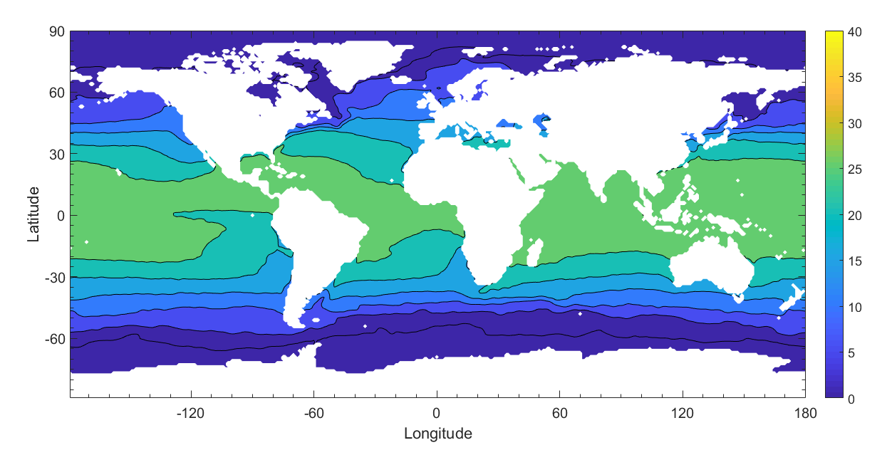
Figure 6: Global annual average of sea surface salinity in parts per thousand (left) and temperature in degrees Celsius (right) for the year 2012.
C. Particle Size Distribution and Global Carbon Flux Estimates
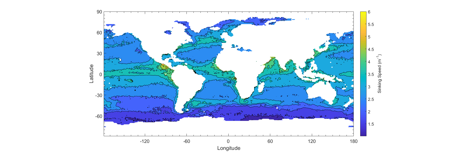
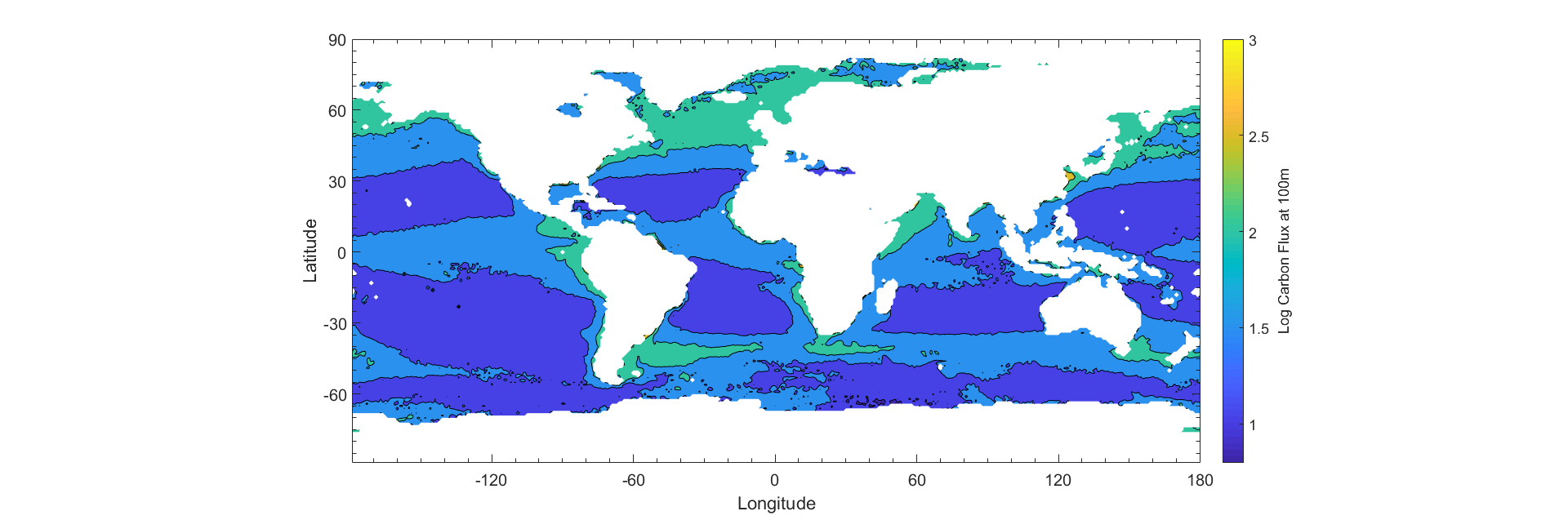
The global distribution of phytoplankton particles can be estimated using satellite data from SeaWiFs (Kostadinov et al 2009). Phytoplankton are ordered into three distinct size classes based on radii. The three size classes are microplankton, nanoplankton, and picoplankton, which are 20 - 50 μm, 2 - 20 μm, 0.5 - 2 μm respectively. These size classes represent percentages of total biomass that each phytoplankton size class contributes to the total. The extended model only applies to diatoms, which have different components of different densities. Because diatoms represent a large population of phytoplankton in the microplankton size class, we treat the size class as a class of diatoms, whereas we treat the other size classes (pico, nano) as following the basic Stokes’ Model. In order to generate an estimate, a weighted average of each size class is input into the respective models using the median radius for each size class (1.25 μm, 11 μm, and 35 μm, for picoplankton, nanoplankton, and microplankton, respectively.) Using the temperature and salinity data, as well as the phytoplankton size fraction (Appendix), we create an estimate of the yearly average sinking speed of all phytoplankton (Fig 7). The total carbon biomass measured from SeaWiFs backscattering (Kostadinov et al 2009) is averaged monthly for the year of 2012. The total biomass is multiplied with the average sinking speed, which gives an estimate of the carbon export (Fig 7.)
Comparisons Between Data
Carbon export data is gathered by deployed neutrally buoyant sediment traps. Our estimated carbon export is compared to observed data gathered at 100m depth (Dunne et al 2005). The observed data offers Our estimated export is compared to the observed data. The data is plotted on a double-log plot (Fig 11) and a linear regression model is fit to the data. The estimated export is weakly correlated with the observed sediment trap data; an R2 value of 0.145. Our estimated product underestimates compared to the observed data by a exponential factor of 2-3, with 80% of the data points falling underneath the 1:1 reference line. The line of best fit plotted against the data has an equation of y = 0.6580x - 0.0742, where the Y axis represents the observed data and the x axis represents the estimated values.
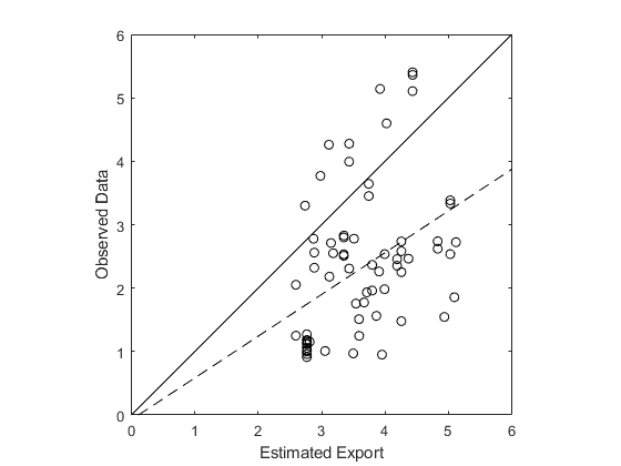 Figure 9: A double-log plot of the estimated export vs sediment trap data (Dunne et al 2005). The solid line pictured is a 1:1 reference line. The dotted line represents the line of best fit for the data. The R2 value for the data is 0.145.
Discussion
The generation of a carbon export estimate from satellite products still has a long way to go. While Stokes’ Law and the extended model presented can be used to explain sinking speed of isolated particles, one limitation is that it cannot be used to explain aggregate structures from satellite derived data. Furthermore, the carbon export estimates are lower than observed and predicted estimates, which may come from a variety of different sources of uncertainty. When compared to in situ data provided by Dunne et al 2005, our estimate has very weak correlation and is extremely noisy. It is uncertain whether the noise is inherent in the data collection process or from the satellite products themselves.
Stokes’ Law is still regarded as a good estimation tool for planktonic sinking speeds. Using the presented extended model can help tighten the overestimation of sinking speeds for larger particles, but is limited to singular particles and cannot account for aggregate phytoplankton structures, which do account for a large portion of carbon export. Aggregate phytoplanktonic structures may also sink very quickly, which is a possible explanation as to why our carbon export estimate is underestimating biomass export despite sinking speeds being overestimated.
Dynamic viscosity has a non negligible effect on sinking speeds. When accounting for both temperature and salinity, over the normal ranges of the physical properties of seawater (0℃ - 40℃ and 30 g / kg - 40 g / kg, for temperature and salinity, respectively), there can be a difference of upwards of 40% increase in sinking speed. The variation in dynamic viscosity is dominated by temperature, which accounts for 86% of the difference in estimated sinking speed at the extremes of temperature and salinity.
There are disparities between sinking speed estimates and carbon export estimates. One of these disparities is that there are high sinking speed estimates at tropical coasts but the export estimates are low. This can be due to less total biomass at the area, which leads to less total carbon export. Additionally, there are areas such as the North Atlantic that do not have abnormally high sinking speeds, but have higher carbon export due to a higher fraction of larger sized plankton and more total biomass.
The total carbon export estimate is found by summing every nonzero element in the monthly average carbon export estimate, and multiplying it by the number of months in a year (12) and the surface area of the ocean (approximately 3.6x10^14 square meters). The estimated yearly carbon export is 0.68 petagrams of carbon, which is about 7.3 times lower than the lowest estimate of carbon export (Smayda 1970). There are several explanations to why the estimate is so low. One explanation may be that since the stokes law model does not apply to large aggregate plankton masses, that the sinking speed and biomass estimates are lower than observed. Furthermore, the satellite products of phytoplankton biomass estimate on the low end of ~0.25 Gt of Carbon (Kostadinov et al 2106). Another explanation to the low estimates may lie in the calculation of the the average sinking speed of phytoplankton. We assume that the microplankton size class is made of entirely diatomic plankton. However, because diatoms are largely cytoplasmic and less dense than traditional phytoplankton particles, the sinking speed averages of microplankton dominated areas may be on the low side.
When comparing our estimates to the observed data, we see very weak correlation and very noisy data. One explanation for the noisy data is that sediment traps are not extremely well developed, leading to some measurements being inconsistent. Sediment traps are also not deployed uniformly, which can result in data is not representative of the total population of phytoplankton. Another potential cause for the noise in data is the satellite driven estimates of phytoplankton size classes and biomass. Satellite data can only capture surface information, and relies on an N0 calibration constant (Kostadinov et al 2016), which is not finalized. The satellite product’s power law algorithm is still fairly new, and is not yet determined to be correct.
Summary and Conclusion
This paper presents both an extended sinking speed estimation method for phytoplankton using dynamic viscosity as well as an estimation process for yearly carbon export from sinking phytoplankton. We use and build upon an extended model created by Miklasz and Denny (2010) in addition to temperature and salinity data from SeaWiFs and Aquarius, respectively. The carbon export estimate presented in this paper is a novel estimation process because it can generate an estimate solely from satellite observations. The estimation process takes particle size distribution data from SeaWiFs that is processed by using only surface layer products, and the carbon export out of the mixed layer can be estimated. However, due to limitations in measuring methods, as well as model limitations, there may be inherent uncertainty. The model presented relies on measurements taken through different satellites and products, and remains a speculative estimate.
Citations
Dunne, J. P., Armstrong, R. A., Gnanadesikan, A., & Sarmiento, J. L. (2005). Empirical and mechanistic models for the particle export ratio. Global Biogeochemical Cycles, 19(4), n/a-n/a. https://doi.org/10.1029/2004gb002390
Kostadinov, T. S., Siegel, D. A., & Maritorena, S. (2009). Retrieval of the particle size distribution from satellite ocean color observations. Journal of Geophysical Research, 114(C9). https://doi.org/10.1029/2009jc005303
Kostadinov, T. S., Milutinovic, S., Marinov, I., & Cabré, A. (2016). Size-partitioned phytoplankton carbon concentrations retrieved from ocean color data, links to data in NetCDF format, supplement to: Kostadinov, Tihomir S; Milutinovic, Svetlana; Marinov, Irina; Cabré, Anna (2016): Carbon-based phytoplankton size classes retrieved via ocean color estimates of the particle size distribution. Ocean Science, 12(2), 561-575 [Data set]. PANGAEA - Data Publisher for Earth & Environmental Science. https://doi.org/10.1594/pangaea.859005
Miklasz, K. A., & Denny, M. W. (2010). Diatom sinkings speeds: Improved predictions and insight from a modified Stokes’ law. Limnology and Oceanography, 55(6), 2513–2525. https://doi.org/10.4319/lo.2010.55.6.2513
Nayar, K. G., Sharqawy, M. H., Banchik, L. D., & Lienhard V, J. H. (2016). Thermophysical properties of seawater: A review and new correlations that include pressure dependence. Desalination, 390, 1–24. https://doi.org/10.1016/j.desal.2016.02.024
Sharqawy, M. H., Lienhard V, J. H., Zubair, S. M. (2010). Thermophysical Properties of seawater: A review of existing correlations and data. Desalination and Water Treatment, 16, 354-380.
http://web.mit.edu/lienhard/www/Thermophysical_properties_of_seawater-DWT-16-354-2010.pdf
Siegel, D. A., Buesseler, K. O., Doney, S. C., Sailley, S. F., Behrenfeld, M. J., & Boyd, P. W. (2014). Global assessment of ocean carbon export by combining satellite observations and food-web models. Global Biogeochemical Cycles, 28(3), 181–196. https://doi.org/10.1002/2013gb004743
Smayda, T. J. 1970. The suspension and sinking of phytoplankton
in the sea. Oceanogr. Mar. Biol.: Ann. Rev. 8: 353–414.